Fractal Dimension CalculatorWritten by Paul BourkeFebruary 2003
Introduction FDC estimates the fractal dimension of an object represented as a black and white image where the object to be analysed is assumed to be made up of the black pixels. This is accomplished by an algorithm called "box-counting". The application provided here is a upgrade to a very popular application written for the Macintosh back in the early 90's. This upgrade is provided for Mac OS-X (as a UNIX application). An earlier application (no longer available) along with the documentation can be found here, in what follows it will be assumed the documentation for the earlier version has been read. Brief theory
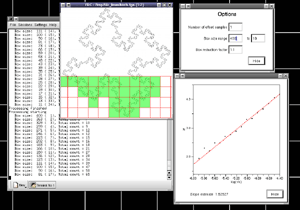
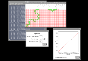
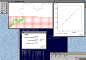
Consider a line, if we subdivide the line in half then it takes two bits to recreate the original line. If we subdivide the line into 4 pieces it takes 4 of them to cover the line. We can write this generally, if we have a line segment of length "s' then the number of segments that will cover the original line is given by N(s) = (1/s)1. Consider a square, if we subdivide it into smaller squares each with 1/2 the side length then it takes 4 of these smaller pieces to form the original square. If we subdivide the square into smaller squares each with 1/4 of the side length then it takes 16 of them to form the original square. As above we can write an expression for the number of pieces we need of size "s" to cover the original square, it is N(s) = (1/s)2. Repeat for a cube....N(s) = (1/s)3. The exponents 1, 2, and 3 in the above examples are fundamental to our concept of the dimension involved. This can be generalised to N(s) = (1/s)D where D is the dimension, an integer as above but it need not be. If we take logarithms of both sides we have log(N(s)) = D log(1/s), in order words we can estimate the dimension by plotting log(N(s)) against log(1/s) the slope of which is the dimension, if it isn't an integer then it's a fractional (fractal) dimension. Screen dumpsA side goal for this project was to see to what extent graphical software could be written and which would compile on multiple UNIX based system including Mac OS-X. The aim was to create a single source version rather than have any special case code for any particular platform. To this end, all the graphics are created using OpenGL and the GLUT interface, all dialogs and user IO is implemented with the Forms (xforms) library. So, it is assumed that OpenGL and X are available, a fairly common situation.
Download FDC is a Mac OSX application that can be freely downloaded for evaluation. It is fully functional except that offset sampling (a critical feature for good estimates of the fractal dimension) isn't enabled. This allows prospective users to check the application runs on their system and performs as expected before investing in a version which will compute more reliable estimates of the fractal dimension. If you have any problems with these demo version please contact the author. To obtain the full version with offset sampling enabled a small fee is payable.
FDC can be run in either graphical mode where the user chooses options and gets graphical feedback on the process or it can be run quietly. FDC will present a window with the current image (it will be empty, white), from here you can use the right mouse button (control click on a Mac with only a single mouse button) to show the menus from where you can open a TGA file (24 or 32 bit), set options, start and stop the processing, display the graph, and save the results for further analysis. The full list of command line options for FDC can be viewed by typing "fdc -h", at the time of writing they are as follows.
Usage: fdc [options]
General options
     -h      this text (help)
     -i s    load input TGA file
     -bw     invert image
     -q      quiet, command line mode
     -p      start processing immediately
Box options
     -n  n   number of offset samples, default: 10
     -b1 n   start box size (default: -1)
     -b2 n   end box size (default: 6)
     -bf n   box reduction factor (default: 1.2)
Region options
     -sl     left boundary (default: 0)
     -sr     right boundary (default: image width)
     -sb     bottom boundary (default: 0)
     -st     top boundary (default: image height)
So for example the command line to run the analysis on the image "snowflake.tga" (supplied in the FDC distribution) quietly with the results written to standard output, using box sizes that range from 200 to 8 in factor steps of 1.2 with 100 offset samples might be as follows. fdc -q -i snowflake.tga -b1 200 -b2 8 -n 100 -bf 1.2 > snowflake.dat The results in "snowflake.dat" will be something like the text on the left below. Where the first column is the box size (s), the second column is the minimum number of covering boxes (N), the third column is log(1/s), and the last column is log(N). The estimate of the fractal dimension is the slope of this graph. If the application is run in graphical mode, at the end of the processing the graph window will look something like the image on the right.
The processing will generally run faster if the options and graph window are hidden. It will run significantly faster if run in "quiet" mode using the "-q" command line option. This is particularly important if a large number of offsets are being used. Box size rangeThe default range of box sizes is usually optimal but not always so. They should only be changed when you have some experience and understanding of the processes involved. The following graph is the result of performing the box counting where the box size ranged from being 5 times the width (or height) of the image to 1 pixel. For successful choice of the box size range it is important to understand the regions of the graph illustrated here. 
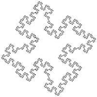
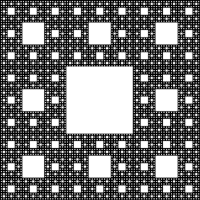
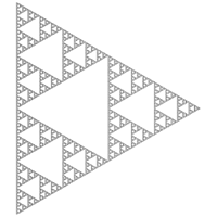
Testing The following are some shapes for which the exact fractal dimension is known, these can test the convergence and the dimension estimated using this software. Note that for the examples below which have a fractal dimension one doesn't expect a perfect match to theoretical because the image is only an approximation to the real fractal form. Note that since FDC assumes the object doesn't exist outside the image area, the estimates for the Sierpinski Carpet are particularly sensitive to this.
Advanced topic: regional analysis
It is possible to analyse just a portion of the image.
For example fdc -sr 700 -sl 400 -sb 300 -st 600 -i gasket.tga 
It is anticipated that in normal operation the area of interest will be chosen in an image editing page prior to analysing the fractal dimension. The ability to process just a region of the image is intended to be used with automatic scripts to estimate the fractal dimension locally across the image, for example, when the dimension is expected to vary across the image. The approach that might be used is to slide a rectangular region across the image estimating the dimension at each position, these estimates can then be combined to form an image showing the dimensional variation. This is similar to a sliding window used in signal processing to calculate the Fourier spectrum variation of a time series. There are two variables involved, the width of the window and the distance between two successive window positions. Typically there is significant overlap between the windows. The image below is formed by analysing a gasket (image size 840 by 950) with a window width of 200 and a window step size of 20. 
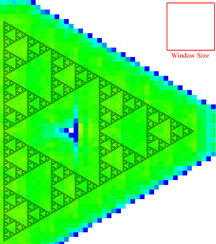
The colour scale is a blue to green to red colour ramp where blue is 1 and red is 2. The correct dimension in this case is 1.585 hence the green appearance. The white region is where the window didn't intersect with any part of the image. 
The window size and stepping are chosen based upon a trade-off between temporal resolution and reliability of the dimension estimate. A large window gives good estimates but low resolution (ability to detect local variations in the dimension), while a small window gives good resolution but poorer estimates. In the example above there are good estimates but low resolution. In the example below a window of 50 is used with the same stepping size of 20, here there is better resolution but poorer estimates. 
Please note that the above colour plots of the sliding window dimension estimates is not part of the FDC package. FDC creates the data for the above but it is up to user to turn that data into a suitable form for visual inspection. Applications of this software
Using Box Counting Techniques for Measuring Shape of Colonies of Filamentous Micro-organisms.
Jacques Soddell and Robert Seviour,
Complexity International (1995) 2
Viscosity of Venusian Lava Flows: Constraints from Fractal Dimension
and Chemical Composition.
W. A. Pike, H.M. Frey, A.E. Krull, E.B. Grosfils, M.S. Gilmore, L.A. Reinen, and S.J. Kozak.
Lunar and Planetary Sciences XX1X
GIS based Compactness measurement Using Fractal Analysis.
Jeffrey L. Knight.
George Mason University Fairfax, Virginia
The Box-Counting: Critical Study.
M. Nezádal, O. Zmeskal, M. Buchnicek.
Technical University of Brno, Faculty of Chemistry,
Institute of Physical and Applied Chemistry,
Purkynova 118, 612 00 Brno, Czech Republic
Fractal Properties of the Thyrotropic Feedback Control
Implications of a Non-linear Model Compared with Empirical Data.
J. W. Dietrich, A. Tesche, C. R. Pickardt and U. Mitzdorf.
Cybernetics and Systems, 2002 Measuring Ocular Redness: First order (luminance & chromaticity) measurements provide more information than second order (spatial structure) measurements. T. Simpson, A. Chan, D. Fonn. Center for Contact Lens Research, School of Optometry, University of Waterloo.
Incident Detection by Fractal Dimension Analysis of Loop Detection Data.
Kim Thomas and Husseun Dia.
22nd Conference of Australian Institutes of transport Research
(CAITR-2000), Ursula College, ANU Campus, Canberra, Australia.
How big is the Milky Way?
+plus issue 15.
Toby O'Neil
Advances in the implementation of the box-counting method of fractal
dimension estimation.
K Foroutan-pour, P Dutilleul, DL Smith.
Applied Mathematics and Computation References Texture Description and Segmentation through Fractal Geometry. J.M. Keller, S.Chen, R.M. Crownover. Computer Vision, Graphics, and Image Processing. 45, 150-166, (1989). The Fractal Geometry of Nature. B.B. Mandelbrot. San Francisco, Freeman. Fractals and Disordered Systems. A. Bunde, S. Havlin. Springer Verlag, Berlin, Heidelberg. The Infinite Number of Generalised Dimensions of Fractals and Strange Attractors. H.G.E.Hentschel, I. Procacaccia. Physica (Amsterdam) 8D, 435 (1983) Determination of Fractal Dimension for Geometrical Multifractals. T. Tel, A. Fulop, T. Vicsek. Physica A, 159, 155-166 (1989)
Ruler or Compass DimensionWritten by Paul BourkeOctober 1998 Update June 2017, see below for an implementation for vector data.
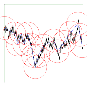
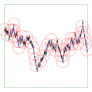
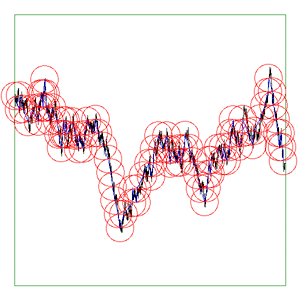
While this application is not generally available, if it is of interest then please contact the author by email. The author is also available for consulting and bespoke software development in this area. Introduction A "standard" method of estimating the length of a curve on a plane is to count how many ruler lengths it takes to move from the start of the curve to the end. Since the ruler has a finite length, the details of the curve that are smaller than the ruler get skipped over and therefore the length we measure is normally less than the real length. This is illustrated below for two rulers (red) of different length being used to estimate the length of the curve in black.  Intuitively we believe that as our ruler gets shorter, our estimate of the real length improves and increases. The estimate of the length on the right image above is closer to the true length because it follows the curve more closely. This improved estimate as the ruler length decreases is certainly true for many curves (1 dimensional objects) but it is not true for others. Such curves are referred to as fractals and they have what is known as a fractal dimension between 1 and 2. Dimension measured in this way is referred to as the Hausdorff Besicovitch dimension. Perhaps the most often quoted example is "How long is the coast of Britain?". One could measure the length using a map and a compass set to say a 50km radius. A better estimate would be achieved by using smaller and smaller compass radii, each one revealing more and more detail. One could go further and have someone walk around the coast, they would still make decisions on how closely they followed the beach. As one became more and more "precise" one would find more and more detail about which to become precise about. As with most fractals in the real world this process and therefore the fractal nature of the object is only appropriate over some limited range of scales. There are many such examples in nature where the relationship between the measured length and the ruler length is not linear, ie: 1 dimensional. The outline of mountain ranges, clouds, and Brownian motion are another examples. The ruler or compass dimension of a curve is computed from the relationship between the length of a ruler and the number of rulers required to measure the length of the curve. This is given by where c is some constant. Taking logs of both sides
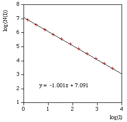
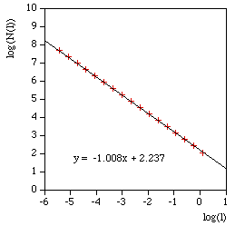
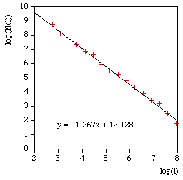
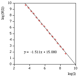
So if we plot log(N(l)) against log(l) for a range of values of l, the slope will be an estimate of the fractal dimension D. ImplementationThe software described here estimates the length of a curve by measuring it with successively shorter ruler lengths. The results when plotted as described above give an estimate of the fractal dimension of the curve.
Note: only continuous curves are possible in this implementation.
The range of line lengths is varied
in powers of sqrt(2) from half the diagonal length of the
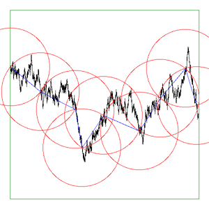
bounding box of the curve to either As the software reduces the ruler it graphically shows the results. The diagrams below are screen snapshots for the first 6 rulers analysing Brownian (1/f2) noise. The black line is the curve being analysed, the blue lines are the ruler lines, and the red lines are the compass radii.
Update: Application to vector data. June 2017
The above are applied to image representation of curves, this can be limiting for many datasets that might have both large scale and fine grain detail thus requiring very large image resolutions to effectively be represented as an image. There are other problems in the reliability of the compass dimension estimates arising from rasterisation of vector data. The software described here (vcompassdim) computes the compass dimension for vector data in 2D. Usage: vcompassdim [options] filename Options -w n Size of output image files, default: do not create The data is conveyed to the software through a text file consisting of x,y pairs, each number and pairs can be separated by any white space character but usually it is a space between x and y and a carriage return before the next pair. The first few lines of an example data file might be as follows 17.3205 90 17.3205 100 25.9808 105 34.641 100 34.641 90 43.3013 95 51.9615 90 51.9615 100 60.6218 105 51.9615 110 51.9615 120 60.6218 125 : : : As per the early fractal dimension estimators, before applying to real data the code should be carefully tested against curves with known dimension. One such curve is the Koch curve with a fracal dimension of log(4)/log(3) = 1.26. A vector form of that curve is generated and the graph of log(l) vs log(N(l)) and linear curve fit shown below. 
As a visual check the software optionally outputs an image for every compass length. As example is shown below, the black line is the curve read from the data file, the blue lines are the rulers following the curve, and the red circles are the compass arcs. 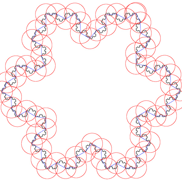
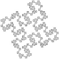
Another example might be to apply to a space filling curve, where the compass dimension should approach 2. An example is below. 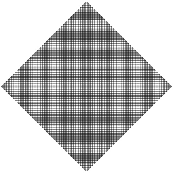
The software writes the log(l) and log(N(l)) as text in 4 columns as follows l N(l) log(l) log(N(l)) 857.369 7 6.75387 1.94591 606.251 21 6.40729 3.04452 428.684 26 6.06072 3.2581 303.126 55 5.71415 4.00733 214.342 116 5.36757 4.75359 151.563 242 5.021 5.48894 107.171 363 4.67443 5.8944 75.7814 810 4.32785 6.69703 53.5855 2186 3.98128 7.68983 37.8907 3280 3.63471 8.0956 26.7928 6561 3.28813 8.7889 18.9454 19683 2.94156 9.88751 13.3964 24907 2.59499 10.1229 9.47268 59049 2.24841 10.9861 6.69819 68890 1.90184 11.1403 4.73634 118098 1.55526 11.6793 And finally the compass dimension is the slope as shown below.

References Andrew Harrison. Fractals In Chemistry, Oxford Chemistry Primers. Oxford Science Publications, 1995 T.G. Smith Jr., W.B. Marks, G.D. Lang, W.H. Sheriff Jr., and E.A. Neal. A Fractal Analysis of Cell Images. Journal of Neuroscience Methods, Vol 27, pp 173-180, 1989 Heinz-Otto Peitgen. Fractals in the Classroom, Part 1. Springer-Verlag, 1991, pp 240 Heinz-Otto Peitgen, Dietmer Saupe. The Science of Fractal Images. Springer-Verlag, pp 61, 1985
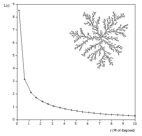
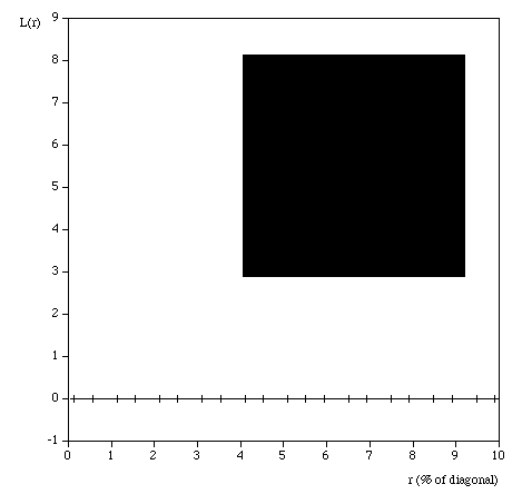
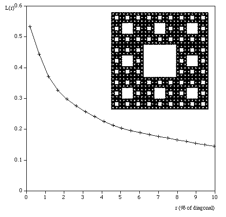
LacunarityWritten by Paul BourkeApril 2004
Lacunarity was initially introduced as a means of further classifying fractals and textures which had the same fractal dimension and a very different visual appearance. Lacunarity is a measure of how the fractal fills space, if the fractal is dense the lacunarity is small, the lacunarity increases with coarseness. Method 1: (Voss)Let P(m,r) be the probability that a box of size r contains m black pixels. Define M1(r) and M2(r) as follows
and
then
Calculate the mean M(r) and variance V(r) of the number of black pixels in each box size r.
 Examples
References Texture Description and Segmentation through Fractal Geometry. J.M. Keller, S. Chen, R.M. Crowover. Computer Vision, Graphics, and Image Processing, 45, 150-166 (1989) Characterisation and measurement to scaling phenomena in disordered systems. R. Voss, R. Pynn and A Skjeltorp, (Ed), New York, 1986. Fractal Methods and Results in Cellular Morphology. G.D. Lange and W.B. Marks. J. Neurosci, 69, 1123-1126 (1996) Lacunarity calculation in the true fractal limit. D.A.Fabio, A. Reis, and R. Riera. J. Phys. A. Math, 27, 1827-1835 (1994) Three-dimensional image analysis and fractal characterization of kidney arterial vessels. M. Sernetz, J. Wubbeke, and P. Wiezek. Physica A, 191: 13-16. (1992)
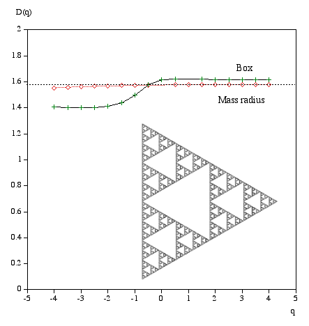
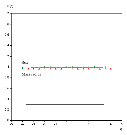
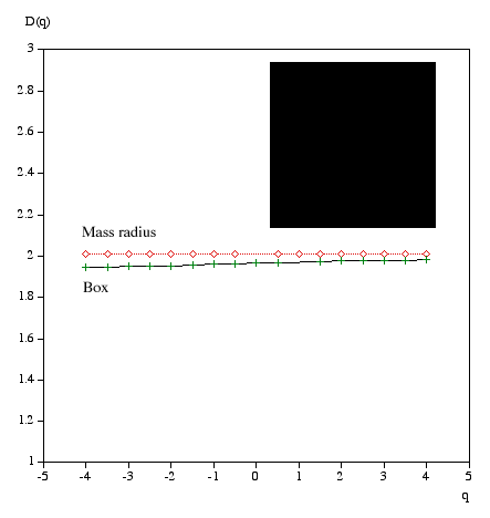
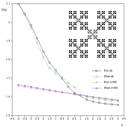
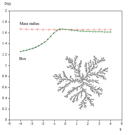
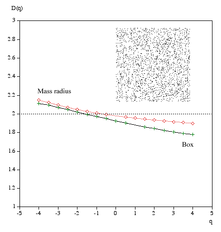
Multifractal spectrumWritten by Paul BourkeJanuary 2004 Box Mass Let N(r) be the total number of boxes (non overlapping) of size length r covering the object. Let Mi(r) be the mass within the i'th box. Define Z(q,r) as follows.
The multifractal dimension D(q) is given by
q ranges from -infinity (concentrates on less dense regions) and +infinity (concentrates on dense regions). For q = 0 this reduces to standard box dimension.
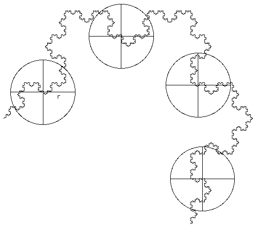
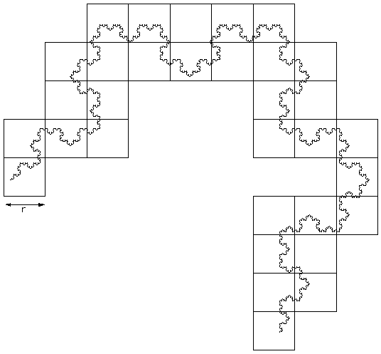 Mass radius Consider all circles of radius r that have their center on the object. Let Mi(r) be the mass within the i'th circle, and the total number of circles of radius r is N(r). Then Z(q,r) is defined as
The multifractal dimension D(q) is given by
 Examples
Multifractal Characterization of Soil Particle-Size Distributions. A.N.D. Posadas, D. Gimenez, M. Bittelli, C.M.P. Vaz, and M. Flury. Soil Sci. Soc. Am. J. 65:1361–1367 (2001) Direct Determination of the f(alpha) Singularity Spectrum. A. Chhabra and R.V. Jensen. Physical Review Letters, 62, March 1989, #12 Multifractal features of random walks on random fractals. A. Bunde, S. Havlin, H.E. Roman. Physical Reviewm A 42, 6274 (1990) Multifractal phenomena in physics and chemistry. H.E. Stanley and P. Meakin. Nature, 335, 405 (1988) Measuring the strangeness of strange attractors. P. Grassberger and I. Procaccia. Physica, Amsterdam, 9D, 189 (1983) Scaling in financial prices: IV Multifractal Concentration. M.B. Mandelbrot. Quantitative Finance, Vol 1, 641-649 (2001) Are Neurons multifractals. E. Fernandez, J.A. Bolen, et al. Journal of Neuroscience Methods, 89, 151-157 (1999) Physical mechanisms underlying neurite outgrowth: a quantitative analysis of neuronal shape. Caserta, F., et al. Physical Review Letters, 1990. 64(1): p. 95-9
Recurrence plotsWritten by Paul BourkeJanuary 1998
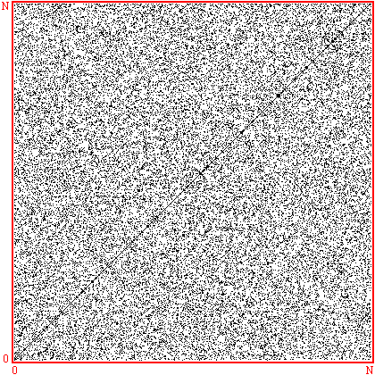
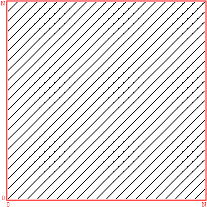
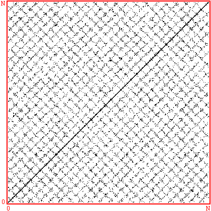
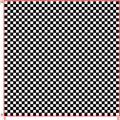
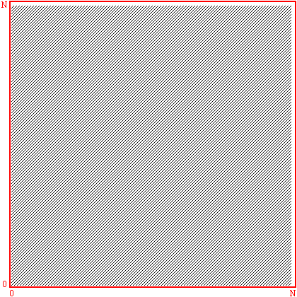
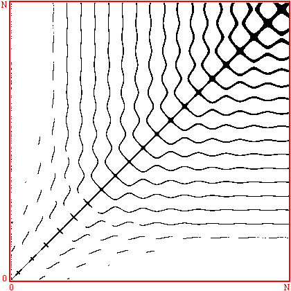
Recurrence plots are used to reveal non-stationarity of a series as well as to indicate the degree of aperiodicity. They were first proposed by Eckmann et al around 1986 in order to study phase space orbits. For example, for a stationary system the recurrence plot should generally be homogeneous along the diagonal. Consider a series x with N terms
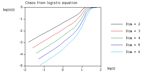
Form all the vectors yi of dimension (length) D with lag (delay) d. D >= 2 and d >= 1 This is normally referred to as embedding x in dimension D with lag d. The recurrence plot is formed by comparing all embedded vectors with each other, and drawing points when the distance between two vectors is below some threshold. More precisely, we draw a point at coordinate (i,j) if the i'th and j'th embedded vectors are less than some distance r apart, eg: a point is drawn if i is plotted along the horizontal axis, j on the vertical axis.
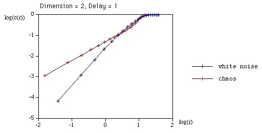
The correlation integral is just the "density" of points on a recurrence plot, that is, the number of points divided by the total number of points in the plot.
Note, the formulation includes the points along the diagonal where i = j. Determining the slope of the correlation integral as a function of log(r) gives the correlation dimension. This is most efficiently computed from a colour recurrence plot where, in general, all the distances have been computed and one simply need to step through a range of radii and count the number of cells with a distance less than the radius.
The usefulness of this result stems from an observation that the fractal
dimension of an attractor of a chaotic system exhibits self similarity.
It can be shown that the topological dimension of an embedding is the
same as the topological dimension of the underlying attractor as long
as the embedding dimension is large enough. Unfortunately there is no
straightforward way to determine what "large enough" is except by
computing the correlation dimension for a number of different embedding
dimensions.
The following illustrative C source was used to generate the diagrams shown above References Understanding Non-linear Dynamics. Daniel Kaplan and Leon Glass. Springer-Verlag Recurrence Plots of Dynamical Systems. Eckman, J.P., et. al. Europhys. Lett. 4, 973 (1 November 1987). Characterization of Strange Attractors. Grassberger, P., Procaccia, I. Phys. Rev. Lett. 50, 346 (31 January 1983).
Self SimilarityWritten by Paul BourkeOctober 2002, updated June 2007
Fractals usually possess what is called self similarity across scales. That is, as one zooms in or out the geometry/image has a similar (sometimes exact) appearance. The following will illustrate various types of self similarity as well as present some real world examples. Exact self similarity
The self similarity may be exact, this normally only occurs in mathematically
defined fractals where the realities/constraints on structures by
the physical world don't apply. The following example is the well
known Koch snowflake curve created by starting with a single line segment
and on each iteration replacing each line segment by four others
shaped as follows 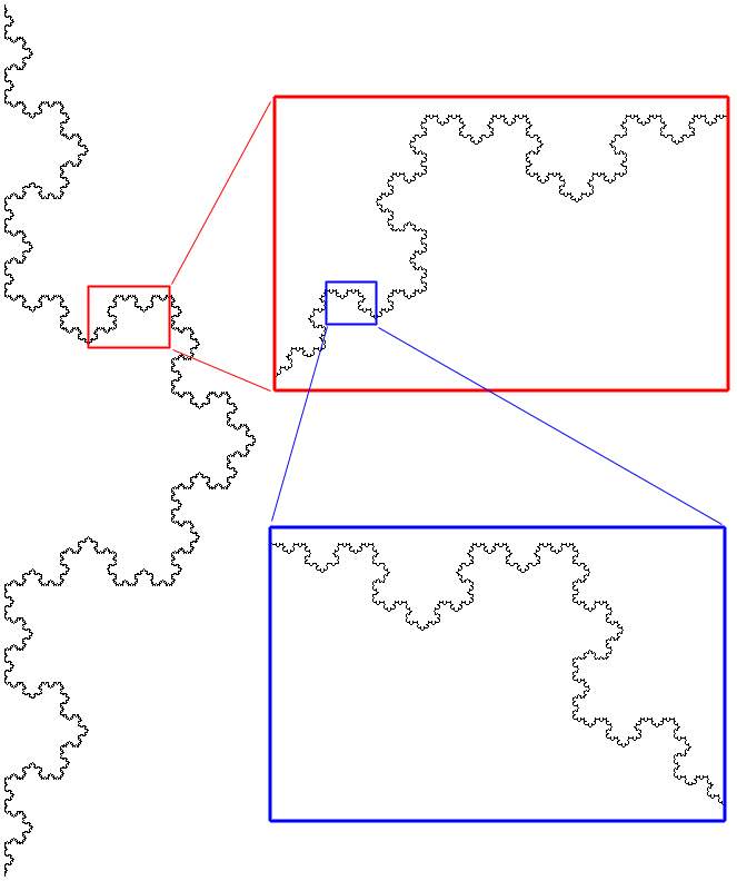
Approximate self similarity A far more common type of self similarity is an approximate one, that is, as one looks at the object at different scales one sees structures that are recognisably similar but not exactly so. An example of this in a mathematically defined system can be readily demonstrated by almost all the patterns seen in the Mandelbrot set. The following show three successive zooms and at each level a structure similar but not exactly the same as the whole Mandelbrot set can be found. 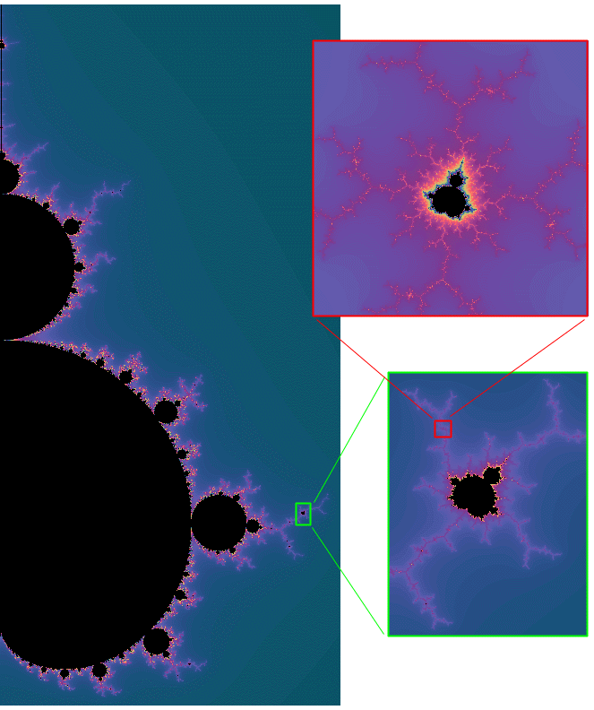
Note that in the above example the self similar structure occurs at discrete levels of scale while other systems like the Koch curve the self similarity occurs at all scales. Statistical self similaritySometimes the self similarity is isn't visually obvious but there may be numerical or statistical measures that are preserved across scales. One obvious measure might be the fractal dimension, in the example below of 1/f noise. the fractal dimension is constant as one zooms in. 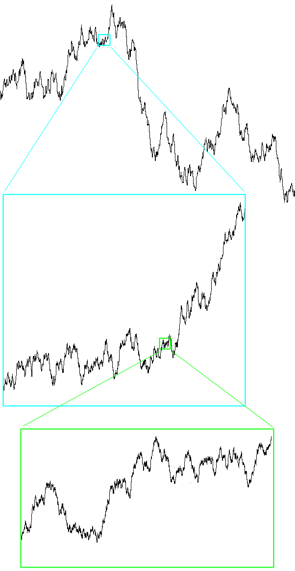
Example 1 - Terrain Consider the following image, is it on the scale of a large piece of rugged terrain photographed from an aeroplane, or the side of a mountain, or a patch of dirt on the scale of a few meters, or a magnification of the surface of a rough rock? Whichever it is, it could also easily be imagined to be any one of the others. So one could start at the large scale view from the air and apply successive zooms down to a microscopic scale, the surface maintains self similarity across those scales. 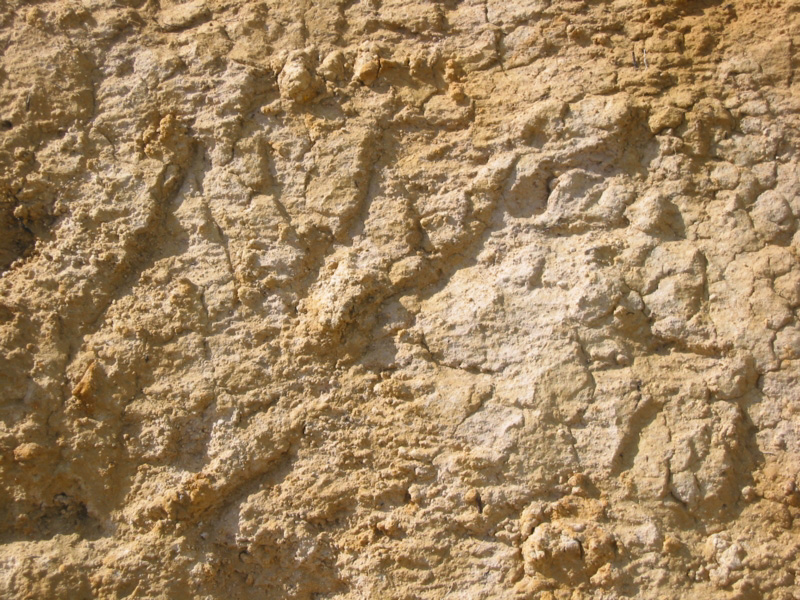
As with most fractal structures found in nature, the self similarity only occurs over a range of scales. In the above example, there is no self similarity as we zoom out to see the whole planet, or zoom in to microscopic scales. Example 2 - Fern leaf
In the case of the self similarity found in the fern, not only is there a limit to the range of scales at which the self similarity occurs but it also occurs at only at a few discrete scales. 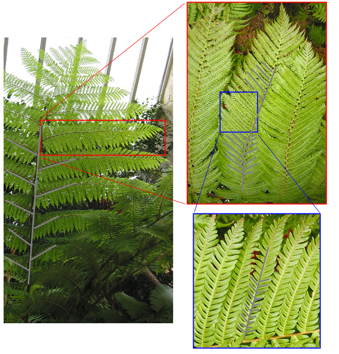 Example 3 - Tree branching
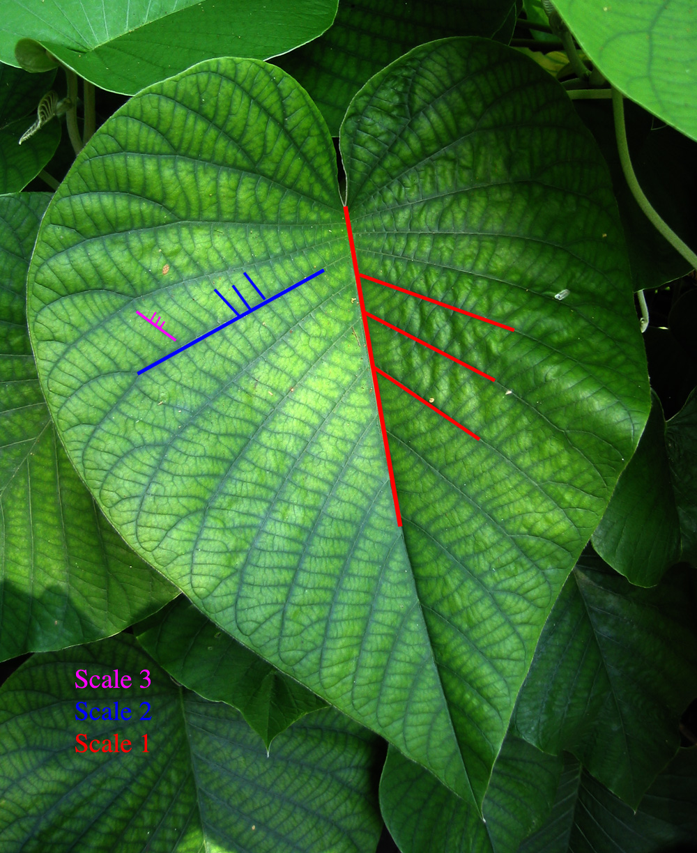
Branching structures such as roots, capillaries, river networks often exhibit self similarity across scales. In some cases, a young tree may be self similar in time, namely, as it grows. A Bonsai tree is a good example (if a little artificial) of this. The trees below, besides the fact that you can see them in their context and thus scale, could easily be imagined to be anywhere in size from a small shrub of 10cm, as they are at about 1m tall, and even as small trees of 10 to 20m in height, or large trees of 100m. They would all pass for possible trees across that large range of scales.
 Tropical leaf |

